Preliminary definitions. Let $r: \mathbb{R} \to \mathbb{R}$ be the firing rate of a neuron, s.t. $r = f \circ g$ for $f: \mathbb{R} \to \mathbb{R}$ a tuning curve and $g: \mathbb{R} \to \mathbb{R}$ a periodic stimulus curve. Assume that $r$ describes the firing rate of a neuron during a trial of length $T$, and let $\Delta t$ be a small positive constant describing the bin size of a partition of $[0, T]$ into $n$ bins.
Spike vector and spike matrix. We define a spike vector as $\omega \in {0, 1}^{n}$ s.t. $\omega_{i} \sim \text{Bernoulli}(r(\frac{i}{T})\Delta t)$. More generally, a spike matrix is defined as a matrix whose rows are spike vectors. The squared spike matrix of $n^2$ dimensions is referred to as the Omega matrix. In other words, we define $\Omega \in { 0, 1 }^{n \times n}$ as a random matrix s.t.
$$ \Omega_{ij} \sim \text{Bernoulli} \Big( r \big( \frac{j}{T} \big) \Delta t\Big) $$
Spike density. Let $\mathcal{D}: \mathbb{N} \to \mathbb{N}$ be the spike density function, defined for $0 < i \leq n$ as
$$ \mathcal{D}(i) = \sum\limits_{j = 1}^{n} \Omega_{ji} $$
where $i =t \cdot T$ with $0 \leq t \leq T$.
Relationship between density and firing rate. The probability that a given value $\Omega_{ij}$ is $1$ is determined by $r(t)$. Let $S_r = \text{sup} { r(t) : 0 \leq t \leq T }$ and $S_{\mathcal{D}} = \text{sup}{ \mathcal{D}(i) : 0 < i \leq n }$. Now observe that
$$ \mathbb{E}\big(\mathcal{D}(i)\big) = \sum\limits_{j=1}^{n} \mathbb{E}(\Omega_{ji}) = nr(t)\Delta t $$
where $t = i/T$. From here it evidently follows that the highest values of $r(t)$ correspond to the highest expected values of $\mathcal{D}$. Informally, the denser regions of $\Omega$ correspond to those around the supremums of $r$.
An application of Frobenius-Perron theorem. By virtue of the Frobenius-Perron theorem, $\Omega$ will have a leading eigenvalue $\lambda$ corresponding to a fully positive eigenvector $\alpha$. Informally, the magnitude of $\lambda$ will be determined by the density of $\Omega$, because each non-null entry in $\Omega$ adds to the magnitude of the linear combination $\Omega \alpha$. The density of $\Omega$ is on its turn dependent on $r(t)$, as was previously observed. It stands to reason that $\lambda$ is dependent on $r(t)$. In particular, $\lambda$ should depend on $S_{r}$ and on the rate at which $r$ dissipates from its peak values as $t$ distances from the values of $S$.
A parameterized rephrasing of the above. Put differently, the leading eigenvalue of $\Omega$ is a random function of the parameters of $f \circ g$. It stands to reason that certain properties of this function may be inferred from the eigenvalue. In general, $f$ may be parameterized to obey a specific maximum $r_{max}$ at some specific stimulus value $s_{max}$ and with a certain decay rate or amplitude $\sigma$. As a mere example, it is conceivable that $f$ should obey a sinusoidal form, and hence may be parameterized as
$$ f(s; r_{max}, \sigma) = r_{max}\sin(\frac{s}{\sigma}) $$
These parameters determine the highest density of $\Omega$ and the rate at which such density dissipates when considering non-maximal time regions.
I simulated a series of spike trains to test whether there is in fact a discernible relation between the Perron eigenvalue of $\Omega$ and the parameters of $f$. For the simulations, I let
$$ \begin{align*} f(s) &= r_{max} \exp \Big( \big( \frac{s-s_{max}}{\sigma} \big)^{2} \Big) \end{align*} $$
This choice is not arbitrary, insofar as this Gaussian curve has been found to fit the firing rate of true biological neurons in the brain. I used two different stimulus curves:
$$ \begin{align*} g_{1}(t) &= \sin(\frac{t}{10}) \newline g_{2}(t) &= \frac{4}{5}t -40 \end{align*} $$
The sinusoidal stimulus was not inspired by any true experiment but chosen due to its convenient and understandable shape. $g_{2}$ is an expression of the rotating light bar experiment detailed in $\text{Part I}$ of Dayan and Abbot's Theoretical Neuroscience. The programming implementation enforced periodicity onto $g_{2}$ so that $g_{2}(T + t) = g_{2}(t)$.
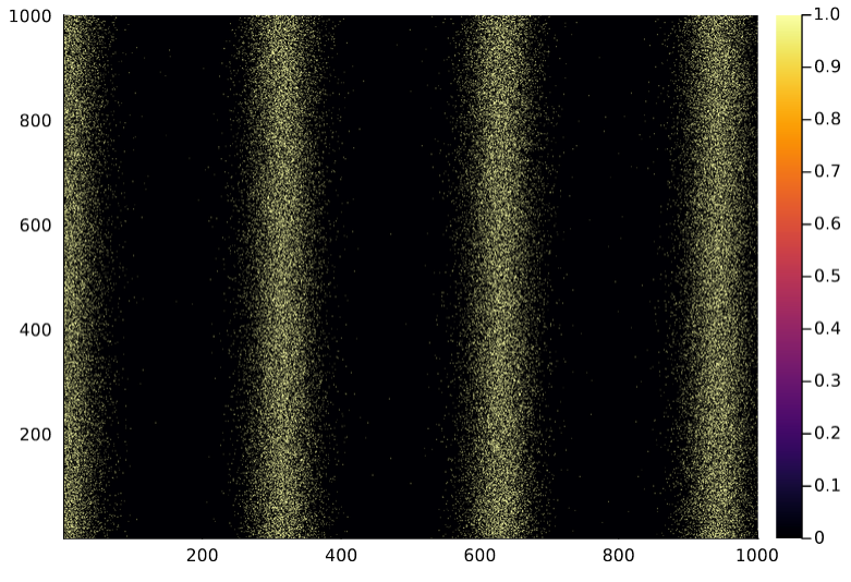
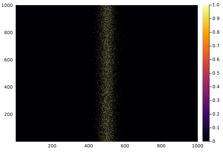
Below is a plot of $\Omega$ under $r_{max} = 4$ and $\sigma = \frac{1}{4}$ for $g_{1}$, followed by a plot of $\Omega$ under $r_{max} = 2$ and $\sigma = 2$ for $g_{2}$.
Under $g_{1}$, the random Perron eigenvalue of $\Omega$ was correctly fitted by
$$ \rho(\Omega) = \sigma r_{max} $$
Under $g_{2}$, it was fitted by
$$ \rho(\Omega)=3\sigma r_{max} $$
Because $\rho(\Omega)$ is a random variable itself, a statistical treatment of it may be useful. But that is a matter of future inquiry.