Adaptive integrate-and-fire neuron model

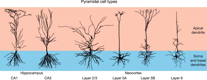
In a Leaky integrate-and-fire neuron model, we discussed a simple model of action potential generation based on Lapicque's work. Some neurons, for example cortical pyramidal cells, show a slight decrease in their firing rate after each spike. This phenomenon is termed spike-rate adaption.

Firstly, recall the basic leaky integrate-and-fire model, where a single leakage current is considered:

$$ \tau_{m} \frac{dV}{dt} = E_{L}-V + R_{m}I_{e} $$

In order to model spike-rate adaption, we add a hyperpolarizing current with a certain conductance $g_{sra}$. This current is modeled as a $K^{+}$ flow with equilibrium potential $E_{K}$.

$$\begin{equation} \tau_{m} \frac{dV}{dt} = E_{L}-V + R_{m}I_{e} - r_mg_{sra}(V-E_{K}) \end{equation}$$

We follow Dayan and Abbot in assuming that this conductance relaxes to zero exponentially obeying

$$\tau_{sra} \frac{dg_{sra}}{dt} = -g_{sra}$$

Observe that

$$ \begin{align*} -\tau_{sra} \int \frac{1}{g_{sra}}dg_{sra} &= \int dt \newline -\tau_{sra} \ln |g_{sra}| +C_1 &= t + C_2 \newline g_{sra}(t) &= A\exp(-t/\tau_{sra}) \end{align*} $$

where $A$ must be defined to satisfy some initial condition when $t = 0$.

Here, $r_m$ determines how strongly the hyperpolarizing current influences the membrane potential. The parameter may be understood to reflect several factors involved in the strength of this current, such as the density of the $K^{+}$ channels that induce spike-rate adaptation.

So far, our added current only counterbalances the external current and thus simply difficults the generation of action potentials. To model spike-rate adaptation, after each spike we increase $g_{sra}$ by a certain amount $\Delta g_{sra}$. We do this specifically by altering the initial condition of $g_{sra}$ (the value of $A$ in its derivation) after each spike. Thus, the hyperpolarizing current increases after each spike, further difficulting the generation of an action potential and thus effectively increasing interspike intervals.

Let us derive the voltage function of this model. Observe that via integration of the equation $\tau_{m} \frac{dV}{dt} = E_{L}-V + R_{m}I_{e} - r_mg_{sra}(V-E_{K})$ we have that

$$ \begin{align*} \tau_m \int \frac{1}{E_L+R_mI_E-V-r_mg_{sra}V+r_mg_{sra}E_K} dV&= \int dt \newline \tau_m \int \frac{1}{V(-r_mg_{sra}-1)+u}dV &= t+C \newline \tau_m \int \frac{1}{Vw+u} dV &= t+C \end{align*} $$

Let $z = Vw+u$ so that $dz = w dV$. Then

$$ \begin{align*} \frac{\tau_m}{w}\int \frac{1}{z} dz &= t+C \newline \ln |z| &= \frac{tw}{\tau_m} + C' \newline z&= A\exp(tw/\tau_m) \end{align*} $$

It follows that

$$ V(t)= \frac{A\exp(tw/\tau_n) - u}{w} $$

If $t = 0$ then $V(0) = (A - u)/w$ from which follows $A= V(0)w+u$.

This is sufficient for us to implement our model. We will use the same parameters as in Leaky integrate-and-fire neuron model for the leaky current. The $K^{+}$ adaptation-inducing current is modeled with a conductance of $100$, $\tau_{sra} = 1, Δg_{sra} = 40, r_{m} = 0.1$ and $E_K = -70$. Except for the equilibrium potential of $K^{+}$, the other parameters were not selected to match real experimental data but rather to clearly show the adaptation.

Note. Yes, this is lousy code. As in previous entries, I only wish to quickly test the theoretical model.

using Plots 

const equilibrium_potential = -65
const membrane_resistance = 10
const external_current = 2
const V₀ = -65
const Vᵣ = -65
const threshold = -50
const τ = 10
const dt = 0.1

const Eₖ = -70
const τₛ = 1
const rₘ = 0.1
const Δg = 40

function gsra(t, gₛ)
    if t == 0 
        return gₛ
    end 

    gₛ * exp(-t/τₛ)
end

function V(t, gₛ)
    if t == 0
        return(V₀)
    end 
    u = equilibrium_potential + membrane_resistance * external_current + rₘ * gsra(t, gₛ)*Eₖ
    w = -rₘ*gsra(t, gₛ) - 1
    
    (V(0, gₛ)*exp(t*w/τ)-u)/w
end

function sim(T, dt, gₛ)
    v = V₀
    values = []
    t = 0
    for i in 0:dt:T
        if v == 1 
            v = Vᵣ  
            push!(values, v)
            t = 0
            gₛ += Δg
            continue
        end
        if v > threshold 
            v = 1 
            push!(values, v)
            continue
        end
        v = V(t, gₛ) 
        t += dt
        push!(values, v)
    end
    plot(0:dt:T, values, xlabel="Time", ylabel="Membrane Potential", label="Membrane Potential")
end

sim(100, 0.1, 100)

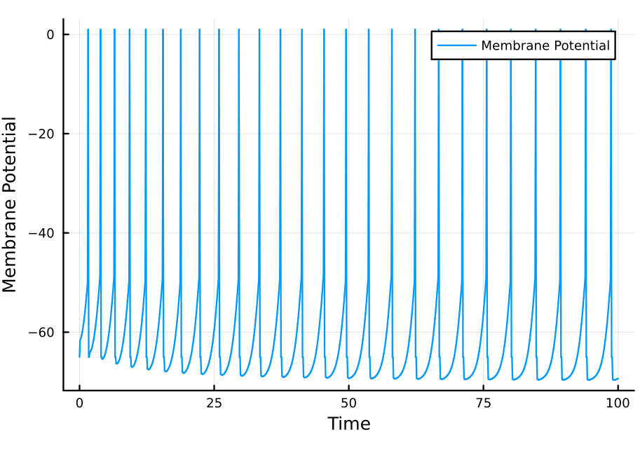
Voilá. Each action potential makes future action potentials more difficult to induce, and the interspike interval increases through time. We have realistically modeled spike-rate adaptation.