In the early twentieth century, Louis Lapicque, a distinguished professor in the Sorbonne and (incidentally) socialist activist, presented the first integrate-and-fire model that described action potentials as induced by a constant current.
Integrate-and-fire models disregard the biophysical subtleties behind action potential generation. Action potentials are assumed to occur whenever the membrane potential $V$ reaches a certain threshold value $V_{th}$. The simplest integrate-and-fire model consists in disregarding all active conductances (including synaptic inputs) and considering only a passive leakage. Hence, it is called the leaky integrate-and-fire model.
Recall that
$$ C_m \frac{dV}{dt} = \frac{dQ}{dt} = -\sum_{ion} I_{ion} + I_{e} $$
where $I_e$ is an external current and $I_{ion} = g_{ion}(V - E_{ion})$. (A more detailed description of these relations is given in Notes on computational neuroscience) Since our model only considers a leaky current, this identity takes the following form in our model:
$$ c_m \frac{dV}{dt} =-g_{leak}(V - E_{leak}) + \frac{I_e}{A} $$
where the external current is divided by $A$, the total area of the neuron, because we are considering the current per unit area (hence the use of $c_m = C_m/A$). If we multiply both sides of this equation by $r_{m}= \frac{1}{\hat{g}_{L}}$, we obtain
$$ \tau_{m} \frac{dV}{dt} = E_{L}-V + R_{m}I_{e} $$
recalling that $r_{m}/A$ is the total membrane resistance $R_{m}$ and $\tau_{m}= c_{m} r_{m}$. This is the essential equation of the leaky integrate-and-fire model. It is easy to derive $V(t)$ from this equation; I will provide this derivation but the reader can skip it and go straight to the result if desired.
$$ \begin{align*} &\tau_m \frac{dV}{dt} = E_L - V + R_mI_e \newline \implies& \frac{\tau_m dV}{u - V} = dt &\{u=E_L+R_mI_e\} \newline \implies& \tau_m \int \frac{1}{u-V}dV = \int dt \newline \implies& -\tau_m \ln |u-V| + C_1 = t + C_2 \newline \implies& \ln |u - V| = -\frac{t}{\tau_m}+C_3 &\{C_3 = C_2 - C_1\} \newline \implies& u-V = Ae^{-t/\tau_m} &\{A = e^{C_3}\} \newline \implies& V=u - Ae^{-t/\tau_m} \end{align*} $$
Solving for $A$ in order to satisfy the initial condition when $t = 0$, we have $A = -(V(0) - u)$, so that
$$ V(t) = u + (V(0) - u)e^{-t/\tau_m} $$
In conclusion, the membrane potential is described in time by the following function:
$$ V(t) = E_L +R_{m}I_{E}+ (V(0) - E_{L} - R_{m}I_{e})\exp(-t/\tau_{m}) $$
It is important to observe that the current $I_{e}$ is assumed to be constant. We will provide later a description of the membrane potential when $I_e$ is itself a non-constant function of time; for the moment, let us try to implement the model.
Implementation: We simulate a neuron with a threshold $V_{th} = -50$mV, $\tau_m = 10$ms, $R_m = 10\text{M}\Omega$, and $E_L = V_{reset} = - 65$mV. The model is implemented in Julia. The model's parameters are given as constants; this is inflexible but our purpose is only to give a quick demonstration.
using Plots

const equilibrium_potential = -65
const membrane_resistance = 10
const external_current = 2
const V₀ = -65
const Vᵣ = -65
const threshold = -50
const τ = 10
const dt = 0.1

function V(t)
    if t == 0
        return(V₀)
    end
    u = equilibrium_potential + membrane_resistance * external_current
    u + (V(0) - u) * exp(-t/τ)
end

function sim(T, dt)
    v = V₀
    values = []
    t = 0
    for i in 0:dt:T
        if v == 1
            v = Vᵣ
            push!(values, v)
            t = 0
            continue
        end
        if v > threshold
            v = 1
            push!(values, v)
            continue
        end
        v = V(t)
        t += dt
        push!(values, v)
    end
    plot(0:dt:T, values, xlabel="Time", ylabel="Membrane Potential", label="Membrane Potential")
end

sim(100, 0.1)
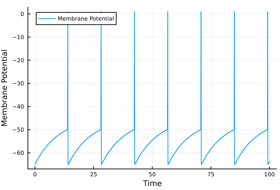
As can be observed in the simulation, because the current $I_e$
(external_current in the program) is constant, the interspike interval is
constant too. It should follow that this interval can be computed analytically,
insofar as it is encoded in the model's equation.
Assume that a spike has occurred at time $t_0$. The next spike will occur at a time $t_{s} = t_0 + \Delta t$ where $V(t_s) = V_{th}$. It follows that
$$ V_{th} = E_L + R_mI_e+(V(0) - E_L - R_mI_e)\exp(-t_{s}/\tau) $$
Solving for $t_s$ and then inverting the result (so as to get the firing rate) we have
$$ r = \frac{1}{t_s} = \Bigg(\tau_m \ln\Big(\frac{R_mI_e+E_L - V_{reset}}{R_m I_e + E_L - V_{th}}\Big)\Bigg)^{-1} $$
If we let $t_0 = 0$ (if we assume a spike occurred instantaneously before the simulation began) then $t_s = \Delta t$ directly provides the interstimulus interval. Observe that in letting $V_{0} = V_{reset}$, as we did in our simulation, we followed this assumption.
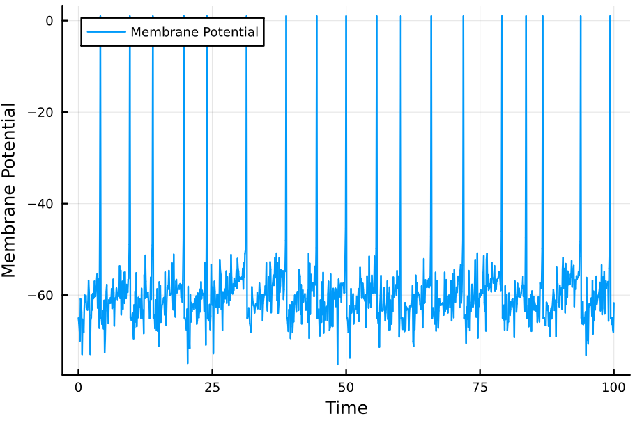
If $I_e$ is not constant, then we must update $V(t)$ not in function of $V(0)$ but in function of $V(t - \Delta t)$ for some small $\Delta t$. In other words, our equation would become
$$ V(t + \Delta t) = E_L+R_mI_e+ \Big( V(t) - E_L - R_mI_e \Big)\exp(-\Delta t/\tau_m) $$
It is straightforward to modify the program above so as to comply with this time-dependence. For example, if we let $I(t) = \cos(t+\Delta t)\sin(t +\Delta t)\times100\sigma$, where $\sigma \sim \mathcal{N}(0, 1)$, the simulation results in
This concludes these quick notes on leaky integrate-and-fire models.