This is a squid neuron firing - or rather an accurate simulation of one. The curve represents the membrane potential of a single neuron, to which an external current is applied from $t = 5$ to $t = 15$. At first glance, the membrane potential might look like a simple spiking curve. However, highly complex biophysical mechanisms are involved in generating this electric fluctuation.
I have reviewed elsewhere a few integrate-and-fire models, such as the Leaky and Adaptive models. These treat the conductance of a given current as a constant $g$ and model action potentials as sudden spikes that appear whenever the membrane potential surpasses a certain threshold. In reality, conductances are not constant and vary with several factors, such as the membrane potential, the influence of neurotransmitters, and other biochemical factors. The seminal Hodgkin-Huxley model deals with voltage-dependent conductances. Curiously, the model was developed studying the squid giant axon.
In this model, which I used to generate the animation above, membrane channels are treated as gating mechanisms that open and close due to voltage-dependent conformational changes in their structure. The "gates" in these channels are comprised of several sub-units, all of which must be in an open state for the gate to be opened. Although the treatment of this gating structures is simple in the model, it reflects actual (but highly complex) cellular mechanisms.
Basic mechanism. As noted in Notes on computational neuroscience, at least two types of voltage-dependent ion channels are required to evoke an action potential in a neuron. Sodium channels open up in response to an increase of the membrane potential—for example, due to the opening of neurotransmitter-gated ion channels and subsequent depolarization—. The influx of $\text{Na}^{\text{+}}$, due to the lower concentration of this ion in the interior of the cell, brings the membrane closer to the sodium resting potential of $\approx +65 \text{mV}$. This is the mechanism behind the rising phase of the action potential. This depolarization provokes two separate but simultaneous phenomena, both occurring about $1 \text{ms}$ after the opening of the sodium channels:
- $i.$ A protein blocks the sodium channels, stopping the influx of this ion;
- $ii.$ Voltage-dependent potassium channels open, and a subsequent efflux of $K^{+}$ drives the membrane potential towards its related potassium resting potential $(\approx -80 \text{mV})$.
The hyperpolarization caused by $ii$ forces both voltage-dependent channels to close, which restores the neuron to its resting state.
Potassium
We will first model potassium channels. The gating mechanism of these channels is modeled as having $k$ sub-units that open and close, so that when all gates are open the ionic current can flow. We let $g_{i} = \bar{g_i}P_i$ where $\bar{g_i}$ is the maximal conductance (the product between the conductance of a single channel of type $i$ and the number of said channels) and $P_i$ is the fraction of channels of type $i$ that are open. Because $P_i$ is a relative frequency it is in fact the probability that a particular channel of type $i$ is open.
Let $n$ be the activation variable, denoting the probability that any given sub-unit of a potassium channel is open. Since all $k$ sub-units must open in order to allow for ions to flow through the channel,
$$ P_K=n^{k} $$
is the probability that the channel is open.
Let $\alpha_n(V)$ be the voltage-dependent opening rate of the sub-units over a small interval of time. Let $\beta_n(V)$ be the closing rate. Naturally,
$$ P(\text{A sub-unit opens}) =\alpha_n(V)(1-n) $$
$$ P(\text{A sub-unit closes}) =\beta_n(V)n $$
The functions $\alpha_n, \beta_n$ are fitted using experimental data. Themordynamical reasons discussed in Dayan and Abbot's book suggest that $\alpha_n$ should be of the form
$$ \alpha_n(V) = A_{\alpha}\exp(-qB_{\alpha}V/k_{B}T) $$
where $\exp(-qB_{\alpha}V/k_BT)$ is the Boltzmann factor. $\beta_n$ should have such form as well though with different constants $A_{\beta}, B_{\beta}$.
Now, we may ask how does the activation variable $n$ vary with time. Naturally, this probability should grow with the probability that sub-units open and fall with the probability that sub-units close:
$$ \frac{dn}{dt} = \alpha_n(V)(1-n)-\beta_n(V)n $$
The equation above states that the probability that a sub-unit is open grows linearly with the probability that sub-units open and falls linearly with the probability that sub-units close.
Note. It is important to understand the difference between $n$ and the rates given by $\alpha_{n}$ and $\beta_{n}$. The activation variable $n$ is the probability that a sub-unit is open. The others are the probability that a sub-unit becomes open or closed, respectively. In other words, the first is the probability of encountering a specific state (open); the others are the probability that a state transition occurs.
If we divide the last equation by $\alpha_{n}(V) + \beta_{n}(V)$, we obtain
$$ \tau_n(V)\frac{dn}{dt} = n_{\infty}(V) - n $$
where $\tau_{n}(V) = 1/(\alpha_{n}(V) + \beta_{n}(V))$ and
$$ \begin{align} n_{\infty}(V) = \frac{\alpha_n(V)}{\alpha_{n}(V) + \beta_{n}(V)} \ \end{align} $$
This is useful because now $dn/dt$ is entirely described in terms of $\alpha_{n}, \beta_{n}$. Furthermore, the first equation states that $n$ approaches the limiting value $n_{\infty}$ exponentially with time constant $\tau_n$. Indeed, for a fixed $V$,
$$ \begin{align*} &\tau_{n} \int \frac{1}{n_{\infty} - n} dn &&= t + C \newline &-\tau_{n}\ln |n_{\infty}-n| +C' &&= t+C \newline &n_{\infty}-n &&= \exp\left(\frac{-t}{\tau_{n}}\right) C'' \newline & n(t) &&=n_{\infty} +\exp\left(-\frac{t}{\tau_{n}}\right) C'' \newline \end{align*} $$
Solving for $C''$ we have
$$ n(t)=n_{\infty}+\exp\left(-\frac{t}{\tau_n}\right)\left(n(0) -n_{\infty}\right) $$
or numerically
$$ n(t +\Delta t) = n_{\infty}+\exp \left( -\frac{\Delta t}{\tau_{n}}\right)(n(t) - n_{\infty}) $$
Since $\exp(-u)$ decreases exponentially to zero, the functional form of $n$ clearly shows how $n$ approaches $n_{\infty}$ indefinitely. From the definition of $n_{\infty}$, it is obvious that this value ranges in $[0, 1]$. This result can be interpreted as follows: At any given voltage level $V$, the probability that a gating sub-unit is in the open state approaches $n_{\infty}$ exponentially. This limiting value is the weight of the opening rate with respect to the transition rate.
Sodium
Sodium channels are modeled as being gated with with two types of gates that open transiently with depolarization. One gate type is the same as the one modeled for potassium channels; their activation variable is termed $m$ and $m^k$ is the probability that said gate is open if it has $k$ sub-units. The second type is a blocker gate that may suppress ionic flow when the other gate is open, and thus the probability $h$ that it is open (not blocking) is termed inactivation variable. This second gating mechanism models the blocking protein described in our summary of the minimal mechanisms behind action potential generation. $m$ and $h$ have opposite voltage dependences; $m$ increases with depolarization and $h$ increases with hyperpolarization. Naturally, the probability that a transient conducting channel is open is given by
$$ P_{Na}=m^{k}h $$
As in the potassium case, $m$ and $h$ are described by rates $\alpha_{m}, \alpha_{h}, \beta_{m}, \beta_{h}$ with similar properties as before. The values used by Hodgkin and Huxley to fit these functions are in page 188 of Dayan and Abbot's book Theoretical neuroscience. As before, the limiting value to which $m, h$ tend is defined as where $z_{\infty}(V)$ with
$$ \begin{align} z_{\infty}(V) = \frac{\alpha_z(V)}{\alpha_{z}(V) + \beta_{z}(V)} \ \end{align} $$
where $z$ can be either $m$ or $h$. Because the functional form of the activation variables are the same, from the derivation of $n(t)$ we can immediately conclude that for any activation variable $z$ we have
$$ z(t)=z_{\infty}+\exp\left(-\frac{t}{\tau_z}\right)\left(z(0) -z_{\infty}\right) $$
or numerically
$$ z(t +\Delta t) = z_{\infty}+\exp \left( -\frac{\Delta t}{\tau_{z}}\right)(z(t) - z_{\infty}) $$
The model
The Hodgkin-Huxley model is based on the channel kinetics we have so far described. The current $I$ is given by
$$ i_{m}=\bar{g_L} (V- E_{L}) + \bar{g_K}n^{4} (V-E_{K) +}\bar{g_{Na}} m^{3}h(V-E_{Na}) $$
The model is implemented using the equation above plus the fact that
$$ c_m \frac{dV}{dt} = -i_m + I_e/A $$
and the equations for each activation variable $z$ with their corresponding limiting values $z_{\infty}$. A possible implementation in Julia is the following:
using Plots

function hh(s, e, T)
    # Maximal conductances used by Hodgkin and Huxley. The order is
    # Potassium, Sodium, Leakage.
    gmax = [36, 120, 0.3]
    # Equilibrium potentials fitted by Hodgkin and Huxley in the same order.
    E = [-77, 50, -54.387]
    I_ext = 0; V = -10; x = [0, 0, 1]; dt = 0.01
    x_plot = []; y_plot = [];
    y_plot_n = []
    y_plot_m = []
    y_plot_h = []
    y_plot_i = []
    for t in range(-30, T, step=dt)
        # Turn external current on or off according to time.
        if t == s  I_ext = 10 end
        if t == e I_ext = 0 end

        # Alpha functions as fitted by Hodgkin and Huxley
        αₙ = 0.01*(V+55)/(1 - exp(-0.1*(V+55)))
        αₘ = 0.1*(V+40)/(1 - exp(-0.1*(V+40)))
        αₕ = 0.07 * exp(-0.05*(V+65))
        α = [αₙ, αₘ, αₕ]

        # Beta functions as fitted by Hodgkin and Huxley
        βₙ = 0.125 * exp(-0.0125*(V + 65))
        βₘ = 4 * exp(-0.0556*(V + 65) )
        βₕ = 1 / (1 + exp(-0.1*(V + 35)) )
        β = [βₙ, βₘ, βₕ]

        # τₓ and x₀, where x₀ is an expression needed to compute
        # the activation variables
        τₓ = 1 ./ (α + β)
        x₀ = α .* τₓ

        # Numerical integration of activation variables
        x = x₀ + exp.(-dt./τₓ) .* (x .- x₀)

        # Compute conductances
        g = [gmax[1] * x[1]^4, gmax[2] * x[2]^3*x[3], gmax[3]]

        # Ohm's law
        I = sum(g .* (V .- E))

        # Update voltage (membrane potential)
        V += dt * (I_ext - I)

        if t >= 0
            push!(x_plot, t)
            push!(y_plot, V)
            push!(y_plot_i, I)
            push!(y_plot_n, x[1])
            push!(y_plot_m, x[2])
            push!(y_plot_h, x[3])
        end
    end
    p1 = plot(x_plot, y_plot, label="")
    ylabel!("V")
    p2 = plot(x_plot, y_plot_n, label="")
    ylabel!("n")
    p3 = plot(x_plot, y_plot_m, label="")
    ylabel!("m")
    p4 = plot(x_plot, y_plot_h, label="")
    ylabel!("h")
    p5 = plot(x_plot, y_plot_i, label="")
    ylabel!("I")
    plot(p1, p2, p3, p4, p5, layout=(5, 1))
    xlabel!("t")
end
To show the behavior of the different factors in the model, I first used the
hh function above to generate a unique action potential. This action potential
is clearly depicted in the voltage $V$ of the membrane in the plot below.
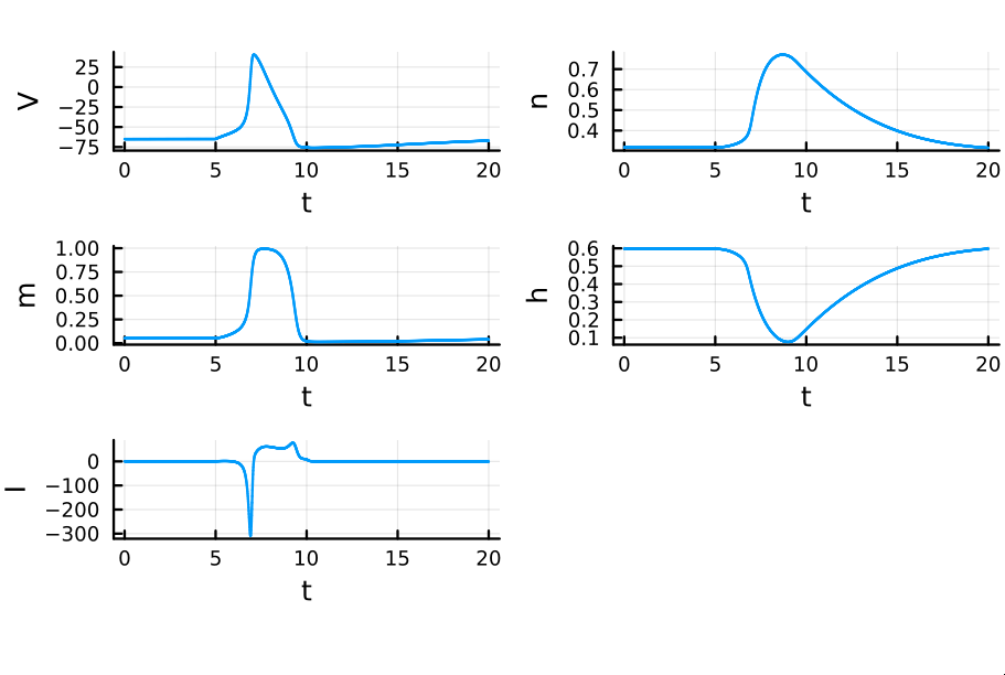
I animated the activation variables using Manim in order to illustrate their reciprocal fluctuations dynamically. The red curve is $n$, the blue curve is $m$, and the white curve is $h$.
Recall that $m$ is the probability that a sodium gating sub-unit (of the first type) is in the open state. The opening of these subunits is the mechanism behind the rising phase of the action potentials. Initially, $m$ is very close to zero and virtually no Na$^{+}$ flow exists. At $t = 5$ we inject an external current, where the rise of $m$ reflects the opening of the sodium channels. For some brief time, just after $m$ rises, both $h$ and $m$ are active; this provokes a sudden influx of $Na^{+}$ ions as reflected in the sharp downward spike of the current $I$. This influx causes the membrane potential to rise close to the equilibrium potential of Na$^{+}$. However, the rise in the membrane potential causes $h$ to fall very close to zero, which reflects the increase in the probability that Na channels are blocked by the blocking protein. This blocking shuts the Na current. Simultaneously, the rise in membrane potential provoked a rise in $n$, which reflects an increase in K$^{+}$. This, combined with the shutting of the Na current, provokes the hyperpolarization observed in the membrane potential.
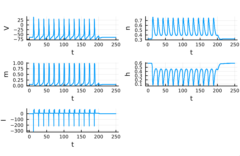
If we do not pause the simulation after the first action potential, but rather perpetuate the external current for a certain amount of time, action potentials are repeatedly generated. Each spike in the simulation below is provoked by the same mechanism as discussed before. The external current was sent from time $t = 0$ to $t=200$.