I presume the reader is familiar at least with the concept of the Fourier transform. Given a function of time $h(t)$, the Fourier transform of $h$ is
$$\begin{aligned} H(f) = \int_{-\infty}^{\infty} h(t) e^{2\pi i f t} ~ dt\end{aligned}$$
This is a representation of $h$ in the frequency domain. If $t$ is measured in seconds, then $f$ is measured in cycles per second, or Hertz. There are interesting relations between $H(f)$ and $H(-f)$, but I skip them because they are not essential to the purpose of this entry.
The most important theorem regarding the total power of a signal is Parseval's theorem:
$$\begin{aligned} \text{total power} \equiv \int_{-\infty}^{\infty} |h(t)|^2 ~ dt = \int_{-\infty}^{\infty} |H(f)|^2 ~ df\end{aligned}$$
The power spectral density (PSD) of $h$ is defined as
$$\begin{aligned} P_h(f) := |H(f)|^2 + |H(-f)|^2 \end{aligned}$$
for $0\leq f < \infty$. When $h(t)$ is real, the two terms are equal and thus we have
$$\begin{aligned} P_h(f) = 2|H(f)|^2\end{aligned}$$
One sometimes sees $P_h(f)$ without this factor of two, but this is only valid when dealing with two-sided spectral densities. We will always deal with the one-sided spectral density.
Sampled data is discrete, but so far we have discussed continuous functions. We need to provide a few concepts before we can extend the Fourier transform to discrete quantities.
For any sampling interval $\Delta$, there is a special frequency called the Nyquist frequency, defined
$$\begin{aligned} f_c := \frac{1}{2\Delta}\end{aligned}$$
If a sine wave with frequency $f_c$ is sampled with sampling rate $\Delta$, then the distance between a peak and a negative trough value is $f_c$.
It is quite easy to observe that if we define the sampling rate as $f_s := \frac{1}{\Delta}$, we have $f_c = \frac{1}{2}f_s$. Sometimes this alternative formulation is given.
The sampling theorem states that if a function $h(t)$ sampled with a rate $\Delta$ happens to be bandwidth limited to frequencies smaller in magnitude than $f_c$, then $h(t)$ is completely determined by its samples $h_n$, and
$$\begin{aligned} h(t) = \Delta \sum_{n=-\infty}^{\infty} h_n \frac{\sin \left( 2\pi f_c(t - n\Delta) \right) }{\pi(t - n\Delta)}\end{aligned}$$
This is nice because it shows that the "information content" of a function that is bandwidth-limited can be totally captured through discrete sampling.
The downside of the theorem is that, when the signal being sampled is not bandwidth limited, the spectral density outside the range $-f_c < f < f_c$ is spuriously movied into that range. This is called aliasing. Aliasing can be avoided if one imposes a bandwidth limit artificially---e.g. via the sampling method---or one samples at a sufficiently small $\Delta$.
The question we know face is that of estiamting $H(f)$ via a discrete sample $h_1, \ldots, h_N$.
With $N$ input values we may only output $N$ values; thus, instead of estimating $H(f)$ for $f \in [-f_c, f_c]$, we may seek estimates only at
$$\begin{aligned} f_n := \frac{n}{N\Delta} \end{aligned}$$
with $n = -\frac{N}{2}, \ldots, \frac{N}{2}$. The equation above gives us the frequency domain of our estimation.
Of course, $H(f)$ is approximated via a discrete sum:
$$\begin{aligned} H_n := \sum_{k=0}^{N - 1} h_k e^{2\pi i k n / N}\end{aligned}$$
Observe that $H_n$, the Discrete Fourier Transform, is independent of any parameter other than the sequence $\left\{ h_n \right\}$, including $\Delta$. When interpreting the result in terms of the sampling frequency, the relationship between the continuous and the discrete Fourier transform is
$$\begin{aligned} H(f_n) \approx \Delta H_n\end{aligned}$$
The discrete form of Parseval's theorem is
$$\begin{aligned} \sum_{k=0}^{N-1} |h_k|^2 = \frac{1}{N} \sum_{n=0}^{N-1} |H_n|^2\end{aligned}$$
There is a famous algorithm, the Fast Fourier Transform, for computing the discrete Fourier transform of a vector. It is a very interesting algorithm that is covered in detail in the book I have referenced. I will not explain it here.
Computing the amplitude spectrum and the power spectrum
The spectral analysis of EEG data typically refers to two things: (1) the power spectrum and (2) its spatio-temporal distribution. I will not concern myself here with spatio-temporal analysis and will only provide simple R functions that estimate the power spectrum. I will provide this functions first with a simulated signal and then use them in an EEG fragment.
The main difficulty in power spectrum density (PSD) estimation over EEG data is the lack of a standard. Different researchers use different methods, and, as I will attempt to show, different methods produce different outputs.
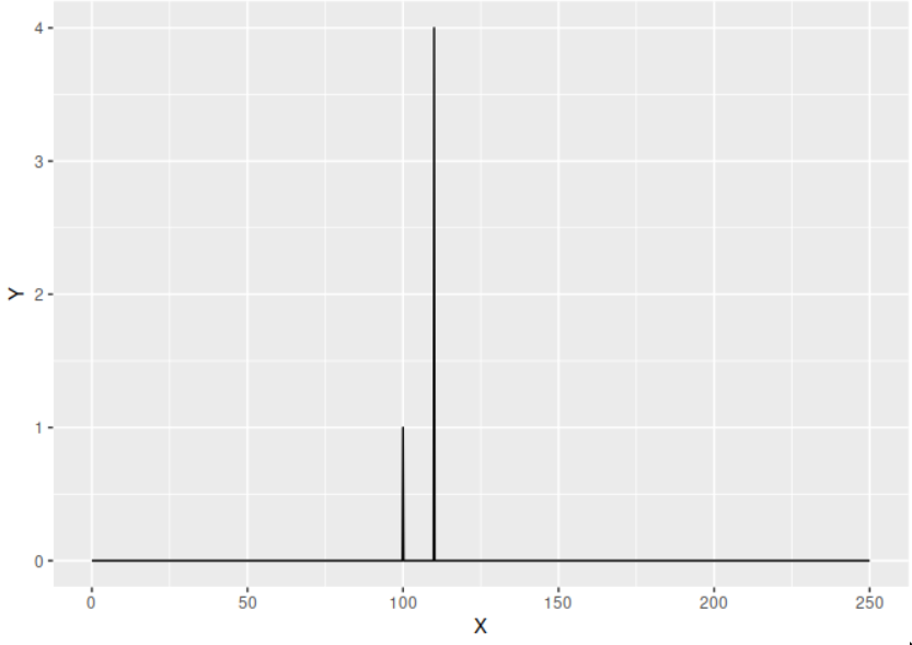
Let's start from the basis and let's simulate the sampling of a simple signal wave in R. The signal we are to simulate is
$$\begin{aligned} h(t) = \sin(2\pi \times 100) + 4 \sin(2 \pi \times 110)\end{aligned}$$
This is, a signal that is a mixture of two sine waves with amplitudes $1$ and $4$, respectively, and frequencies $100$ and $110$, respectively.
    set.seed(123)

    # Parameters
    sampling_rate <- 500 # Sampling rate (samples per second)
    duration <- 5-1/sampling_rate           # Duration of the signal in seconds
    frequencies <- c(100, 110)  # Frequencies of the sine waves (in Hz)
    amplitudes <- c(1, 4)   # Amplitudes of the sine waves

    # Generate time vector
    t <- seq(0, duration, by = 1/sampling_rate)
    n <- length(t)

    # Initialize signal as zeros
    signal <- rep(0, n)

    # Create a signal as a mixture of sine waves
    for (i in seq_along(frequencies)) {
      frequency <- frequencies[i]
      amplitude <- amplitudes[i]

      # Generate the sine wave component
      sine_wave <- amplitude * sin(2 * pi * frequency * t)

      # Add the sine wave component to the signal
      signal <- signal + sine_wave
    }
The amplitude spectrum of the signal is given by
$$\begin{aligned} P(f) = \frac{2|H(f)|}{N}\end{aligned}$$
which is easily computed in R.
    my_amplitude <- function(x, sampling_rate){
        N <- length(x)
        ft <- abs(fft(x)) # Absolute value of the FFT.
        ft <- ft[1:(N/2 + 1)] # Make one sided.
        freq <- c(0:(length(ft)-1))*sampling_rate/length(x) # Compute the frequency domain.
        amplitude <- 2/N * ft
        return(list(freq = freq, amplitude = amplitude))
    }
amp <- my_amplitude(signal, sampling_rate = 500)
ggplot(data.frame(X = amp$freq, Y = amp$amplitude), aes(x = X, y = Y)) + geom_line()
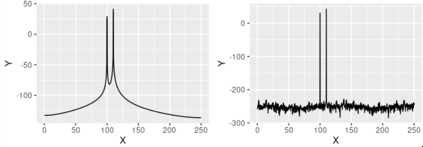
The PSD is defined as
$$\begin{aligned} P(f) = \frac{2|H(f)|^2}{W}\end{aligned}$$
where $W = \sum_{i=0}^{N-1} w_i^2$ and $w_0, \ldots, w_{n-1}$ is the window function used. If no window is used, this is equivalent to a rectangular window and $W = N$. In R, this is again straightforward to compute:
    my_psd <- function(x, sampling_rate, han = TRUE){
        N <- length(x)
        if (han){
            hann <- gsignal::hann(N) # Hanning window
            x <- x * hann
            normalization <- 2/(sum(hann^2))
        }else{
            normalization <- 2/(N) # Rectangular window
        }
        ft <- abs(fft(x))
        ft <- ft[1:(N/2 + 1)] # Make one sided
        freq <- c(0:(length(ft)-1))*sampling_rate/length(x) # One sided fft

        power <- ft^2 * normalization
        return(list(spec = power, freq = freq))
    }
Sometimes, one sees
$$\begin{aligned} P(f) = \frac{2|H(f)|^2}{W \times f_s}\end{aligned}$$
It is important to note that $f_s$ here is a scaling factor that translates from units of power to units of power/Hz. This is useful when comparing powers from signals with different sampling rates. The power spectrum (in decibels) of our signal, with and without a Hanning window, is the following.
psd1 <- my_psd(signal, sampling_rate = 500, han = TRUE)
psd2 <- my_psd(signal, sampling_rate = 500, han = FALSE)
p1 <- ggplot(data.frame(X = psd1$freq, Y = gsignal::pow2db(psd1$spec)), aes(x = X, y = Y)) + geom_line()
p2 <- ggplot(data.frame(X = psd2$freq, Y = gsignal::pow2db(psd2$spec)), aes(x = X, y = Y)) + geom_line()
cowplot::plot_grid(plotlist=list(p1, p2))
Welch's method
I provide a quick implementation of Welch's method. Welch's method consist of splitting the signal $h(t)$ into $K$ overlapping segments of length $L$, where the overlap is defined as a percentage of the segment length (and hence falls within $0$ and $1$). A slightly modified estimation of the power spectral density is computed for each segment, and then the estimations of all segments are averaged. The estimation in each segment, according to the original paper , is done as follows:
-
For each segment $s_i(t)$ of length $L$, compute $F_i := \frac{1}{L}S_i(f)$, where $S(f)$ is the Fourier transform of $s_i$, and $f = \frac{n}{L}$ for $n = 0, 1, \ldots, \frac{L}{2}$.
-
Compute $U := \frac{1}{L} \sum_{i=0}^{L-1} w_i^2$ with $w_0, \ldots, w_{L-1}$ the window function.
-
Compute $\frac{L}{U} |F_i|^2$
This results in the power spectrum of the segment in question. If everything is put together, and we add a factor of two to account for the one-sided spectrum (this is not the case for the original paper), the power spectrum of each segment is
$$\begin{aligned} A_i = \frac{2L}{U} \left[ |\frac{2}{L} S_i(f)| \right]^2 = \frac{2}{LU}|S_i(f)|^2 = \frac{2|S_i(f)|^2}{\sum w_i^2}\end{aligned}$$
This expression is prettier to program. In R,
    overlaps <- function(signal, L, D){
        # Calculate the number of segments
        D <- L * D
        M <- ceiling((length(signal) - L) / (L - D)) + 1

        # Initialize a list to store segments
        segments <- list()

        # Create overlapping segments
        for (i in 1:M) {
          start <- (i - 1) * (L - D) + 1
          end <- start + L - 1
          if (end > length(signal)) {
            break
          }
          segments[[i]] <- signal[start:end]
        }
        return(segments)
    }

    my_pwelch <- function(signal, sampling_rate, L, D){


        modified_periodogram <- function(segment){
            L <- length(segment) # L to distinguish that this is the length of a segment, not the whole (original) signal!
            hann <- gsignal::hann(L) # Hanning window
            x <- segment * hann
            ft <- fft(x) # Aₖ(n)
            ft <- ft[1:(L/2 + 1)] # Lake one sided
            w <- 2*abs(ft)^2/sum(hann^2)
            freq <- c(0:(length(ft)-1))*sampling_rate/L
            return( list(freq = freq, spec = w) )
        }

        segments <- overlaps(signal, L, D)
        m_periodograms <- lapply(segments, modified_periodogram)
        spectrums <- lapply(m_periodograms, function(x) x$spec)
        n <- length(m_periodograms) # Number of segments
        avg_spectrum <- 1/n * rowSums(do.call(cbind, spectrums))
        return ( list(freq = m_periodograms[[1]]$freq, spec = avg_spectrum))
    }
Here's a comparison of what results from our own my_pwelch function and
the pwelch function from the gsignal package.
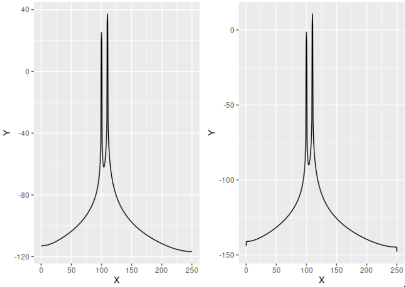
The difference in the scales comes from the fact that gsignal's pwelch function
adds a factor $1 / f_s$ to the normalization (i.e. its output is not in units of
power but of power/Hz). I have verified that adding this factor to my function
yields the exact same result.