Introduction
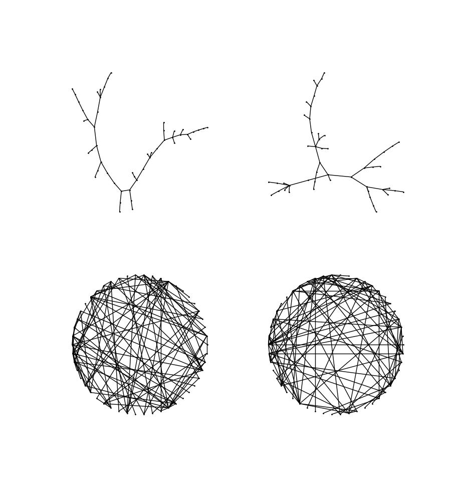
The generation of connected random graphs is non-trivial and important to many applications. In general, given $n, m \in \mathbb{N}$, it is not difficult to sample a random graph from the space of all graphs of $n$ vertices, $m$ edges. The problem becomes more difficult when we require (a) that the randomly generated graph be connected and, if possible, (b) that any possible such graph has the same probability of being generated (i.e., that we sample the connected graphs uniformly).

A direct and simple algorithm is to generate a random tree (e.g., via a Prüfer sequence) and add edges randomly until the desired number of edges is reached.
This procedure is relatively efficient ($\mathcal{O}(n^2)$), but it is biased. Not all connected graphs have the same number of spanning trees, and therefore the probability of generating a given connected graph is not uniform.
A computationally heavier approach is to generate a $K_n$ and prune edges randomly until the desired number of edges is reached, while maintaining the connectivity invariant. This algorithm is unbiased, but its complexity is higher. The procedure is as follows:
- $(V, E) := \mathbf{genKn}(n)$
- $E_c := [e_1, \ldots, e_{|E|}]$
- while $|E| > m$ do
- ${v, w} := \mathbf{randSample}(E_c)$
- $E := E - {v, w}$
- if $\neg \mathbf{ConnectivityCheck}(E, v, w)$ then
- $E := E \cup {v, w}$
- $E_c := E_c - {v, w}$ (edge is a bridge)
- return $(V, E)$
Generating a $K_n$ is $O(n^2)$. The while loop selects a random edge from $E_c$ and attempts to prune it. There is only one case in which an edge is not removed; namely, when the sampled edge is a bridge. This happens at most once per bridge. There are at most $n - 1$ bridges in a graph. Hence, there are $O(n)$ iterations which do not remove an edge.
The remaining iterations will remove an edge and there will be exactly $\frac{n(n-1)}{2} - m$ of them.
Therefore:
$$ O(n) + O\Big(\frac{n(n-1)}{2} - m\Big) = O(n^2 - m) $$
iterations.
The operations in each iteration are $O(1)$ except the connectivity check, which we assume to be a BFS search with starting vertex $v$ and target vertex $w$. BFS is $O(n^2)$.
Therefore:
$$ O(n^2) + O(n^2 - m)O(n^2) = O(n^4 - n^2m) $$
In practice, the algorithm will perform better than this. BFS stops whenever $w$ is found starting from $v$. This still is asymptotically $O(|E|)$, but in practice the bound will seldom be reached. Furthermore, BFS is run on increasingly sparser graphs.
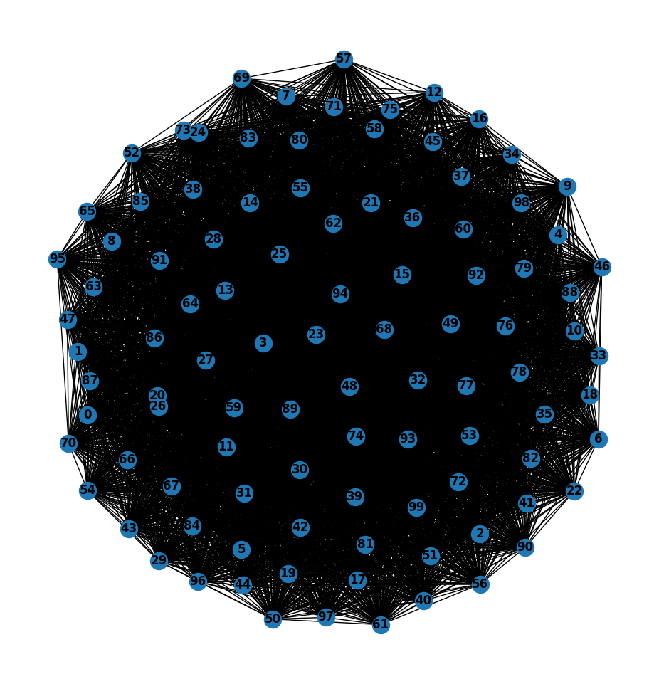
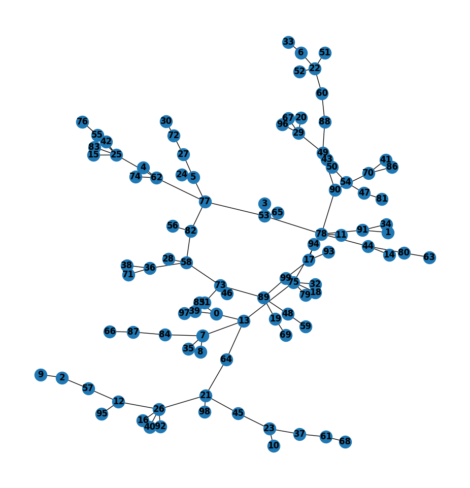
Below, I display a $K_{100}$ and the random tree generated from it.


Correctness and uniformity
To prove that the algorithm is unbiased we need a few definitions.
Let $\mathcal{G}_{n, m}$ denote the set of all graphs with $n$ vertices and $m$ edges, and let $\mathcal{C}_{n, m} \subset \mathcal{G}_{n, m}$ denote the subset of connected graphs.
Let $\mathcal{E}_{n,m}$ be the class of edge sets $W \subseteq E(K_n)$ such that removing $W$ from $K_n$ produces a connected graph with $m$ edges.
Each $G \in \mathcal{C}_{n, m}$ corresponds uniquely to one such $W \in \mathcal{E}_{n,m}$, so
$$ |\mathcal{E}_{n,m}| = |\mathcal{C}_{n, m}| $$
It follows that there is a bijection
$$ f_{n,m} : \mathcal{E}{n,m} \to \mathcal{C}{n, m}, \quad f_{n,m}(W) = (V, E(K_n) - W). $$
We now prove that:
- The edges removed by the algorithm form a valid set $W \in \mathcal{E}_{n,m}$ and the resulting graph is $f_{n,m}(W)$.
- Each $W \in \mathcal{E}_{n,m}$ may be formed with equal probability.
(1) Correctness
The algorithm removes $k = \binom{n}{2} - m$ edges
$$S = \{ e_1, \ldots, e_k \}$$
The connectivity invariant is preserved at each successful removal, so
$$ \{ e_1 \}, \{ e_1, e_2 \}, \ldots, \{ e_1, \ldots, e_k \} \subseteq \mathcal{E}_{n, m} $$
By construction, the final graph has edges $E(K_n) - S$, i.e. the final graph
equals $f_{n,m}(S)$.
∎
(2) Unbiasedness (symmetry argument)
The algorithm removes the edges of some $W \in \mathcal{E}_{n,m}$ and each successful run corresponds to an ordered sequence $(e_1,\dots,e_k)$ which is a permutation of the elements of that $W$.
-
If $W\in\mathcal{E}_{n,m}$, then for any subset $S'\subseteq W$ the graph $f(S')$ is still connected (removing fewer edges cannot disconnect a graph that remains connected after removing the larger set). Hence any permutation of the $k$ edges of $W$ is an admissible removal order: none of those edges will ever be a bridge at the moment it is removed. Therefore, the number of admissible orders that produce $W$ is exactly $k!$.
-
By vertex- and edge-symmetry of $K_n$, the size $|E_i|$ of the candidate set at step $i$ depends only on $i$ (and on $n,m$), not on which particular edges form $S_{i-1}$. Denote $a_i:=|E_i|$.
At step $i$, the algorithm chooses uniformly from $E_i$, so the probability of that exact ordered sequence is:
$$ \prod_{i=1}^k \frac{1}{a_i}. $$
Since there are $k!$ ordered sequences (permutations) that yield the same unordered set $W$, the probability of producing $W$ equals:
$$ P[\text{output } W] = k! \prod_{i=1}^k \frac{1}{a_i}. $$
The right-hand side does not depend on $W$ (only on $k$ and the sequence $a_i$), so every $W\in\mathcal{E}_{n,m}$ is produced with the same probability. Thus, the induced distribution on $\mathcal{C}_{n, m}$ is uniform — the algorithm is unbiased.
As a Markov Chain
Let $G_i$ denote the graph after $i$ successful iterations of the edge-pruning algorithm. Then the sequence $\{G_i\}_{i\ge 0}$ defines a discrete-time Markov chain (DTMC) on the state space $\mathcal{C}_{n, m}$, the set of connected graphs with $n$ vertices and $m$ edges.
Markov property
The Markov property holds because the choice of edge to remove at step $i+1$ depends solely on the current graph $G_i$ and the remaining candidate edges $E_c$. Formally:
$$ P[G_{i+1} \mid G_i, G_{i-1}, \dots, G_0] = P[G_{i+1} \mid G_i]. $$
Transition probabilities
Let $P(G_i \to G_{i+1})$ denote the one-step transition probability from graph $G_i$ to graph $G_{i+1}$, assuming $G_{i+1} \neq G_i$. Then:
$$ P(G_i \to G_{i+1}) = \begin{cases} \frac{1}{|E_i|}, & \text{if $G_{i+1}$ can be obtained by removing a single non-bridge edge from $G_i$,}\ 0, & \text{otherwise.} \end{cases} $$
If a sampled edge is a bridge, then the graph remains unchanged and $G_i =G_{i+1}$. The probability of this self-loop transition is:
$$ P(G_i \to G_i) = \frac{|B_i|}{m_i}, $$
where $B_i$ is the set of bridge edges at the current iteration and $m_i$ is the number of edges in $G_i$.
Note that $B_i = \overline{E_i}$, which means:
$$ P(G \to G) = \frac{m_i - |E_i|}{m_i} = 1 - \frac{|E_i|}{m_i}. $$
From this follows that the probability that an edge is successfully removed at iteration $i$ is $|E_i| / m_i$.
Note that there are at most $n-1$ bridges in a connected graph with $n$ vertices, and this bound remains constant across iterations, so:
$$ P(\text{A bridge is chosen at iteration } i) \leq \frac{n-1}{m_i}. $$
This bound is informative only when $m_i \gg n - 1$, since otherwise it approximates 1 and becomes trivial. Thus, it is informative for dense graphs and not for sparse ones.
Stationary distribution
Since the algorithm is unbiased, every connected graph $G \in \mathcal{C}_{n,m}$ is equally likely to appear as the final output. This implies that the stationary distribution $\pi$ of the Markov chain is uniform over $\mathcal{C}_{n, m}$:
$$ \pi(G) = \frac{1}{|\mathcal{C}_{n, m}|}, \quad \forall G \in \mathcal{C}_{n, m}. $$
Irreducibility and aperiodicity
The chain is irreducible in the sense that, starting from $K_n$, any connected graph with $m$ edges can eventually be reached by a sequence of valid edge removals.
The chain is aperiodic because there is a positive probability of staying in the same state (when a bridge is sampled):
$$ P(G \to G) > 0 \quad \forall G \in \mathcal{C}_{n, m}. $$
Hence, the Markov chain converges to the uniform stationary distribution.
A potential improvement
The probability that a chosen edge is a bridge increases as the graph becomes sparser, but is relatively negligible in the early stages of the algorithm. Since such probability is bounded at each iteration by $ (n-1)/m_i $, and both of these quantities are known to the algorithm, we can define a tolerance $ \epsilon $ such that if
$$ \frac{n-1}{m_i} < \epsilon, $$
we skip the connectivity check and automatically remove the sampled edge.
Appendix
As an appendix, let us derive the number of connected graphs of $n$ vertices, $m$ edges. Note that
$$ \begin{align*} |\mathcal{G}_{n, m}| = \binom{\frac{n(n-1)}{2}}{m} \end{align*} $$
This inspires the definition of a generating function for the class $\mathcal{G}_{n, m}$ of graphs of $n$ vertices, $m$ edges:
$$ \begin{align*} A(z, u) &= \sum_{k=0}^{\infty}\left(\sum_{r = 0}^{\infty} \binom{\frac{k(k-1)}{2}}{r} u^r\right) \frac{z^k}{k!}\\ &=\sum_{k=0}^{\infty}(1 + u)^{\frac{k(n-1)}{2}} \frac{z^k}{k!} \\ &= 1 + \sum_{k=1}^{\infty} (1+u)^{k(k-1)/2} \frac{z^k}{k!} \end{align*} $$
An important observation is that any $G \in \mathcal{G}_{n,m}$ is a set of elements $G_1, \ldots, G_r \in \mathcal{C}_{n, m}$. Informally, any graph is a set of connected graphs. Since the relationship of the class $\mathcal{G}_{n, m}$ and the class $\mathcal{C}_{n, m}$ is the set-of relation, the generating function $C(z, u)$ of $\mathcal{C}_{n,m}$ is satisfies
$$A(x) = e^{C(z, u)} $$
Then
$$ \begin{align*} C(z, u) &= \ln \left[1 + \sum_{k=1}^{\infty} (1+u)^{k(k-1)/2} \frac{z^k}{k!}\right] \\ &= \sum_{q=1}^{\infty} \frac{ (-1)^{q+1} }{q} \left[ \sum_{k=1}^{\infty}\left( 1+u \right)^{k (k-1) / 2} \frac{z^k}{k!} \right]^{q} \end{align*} $$
Thus, $C(z, u)$ is the generating function of the composite sequence $\{\{|\mathcal{C}_{n, m}|\}_{n\geq 1}\}_{m\geq 0}$. The resulting expression for the number of connected graphs of $n$ vertices, $m$ edges is:
$$ \begin{align*} \mathbb{C}(n, m) = n! ~ [ z^n ][ u^m ] \sum_{q=1}^{\infty} \frac{ (-1)^{q+1} }{q} \left[ \sum_{k=1}^{\infty}\left( 1+u \right)^{k (k-1) / 2} \frac{z^k}{k!} \right]^{q} \end{align*} $$
where $[z^n][u^m]C(z, u)$ are the $n$th and $m$th coefficients of the generating functions for the polynomials dependent on $z$ and $u$, respectively.
Example. For $m = n - 1$ (i.e. connected trees) across $n = 2, 3, \ldots$, $\mathbb{C}$ effectively produces the sequence
$$ 1, 1, 3, 16, 125, 1296, \ldots = {n^{n-2}}_{n\geq2 }$$
which we know is correct because there are $n^{n-2}$ Prufer sequences of length $n$.