Let $X(t), Y(t)$ denote two signals viewed as random variables. Their cross-correlation is defined as
$$(X \star Y)(\tau) = \int_{-\infty}^\infty X(t)Y(t + \tau) ~ dt$$
As a simple note, we observe that for $\tau = 0$ their cross correlation becomes $\int_{-\infty}^\infty X(t) Y(t) ~ dt = \mathbb{E}\left[ X \cdot Y \right]$. If $X, Y$ are zero-meaned then this entails $(X \star Y)(0) \propto \text{Cov}(X, Y)$. In short, the zero-lag cross-correlation of two zero-mean signals is proportional to their covariance.
For discrete signals, like digital EEGs, the definition is analogous, though this time we normalize:
$$ \begin{align*} C(t) = \frac{1}{(N-m)\sigma_X \sigma_Y} \sum_{j=0}^{N-(m+1)} \hat{X}_j \hat{Y}_{j+m}, \qquad t = m\tau \end{align*} $$
where
-
$\hat{X}_i$ is the fluctuation of $X_i$ around its mean ($X_i - \bar{X}$);
-
$\tau$ is the constant sampling time, i.e. the inverse of the sampling rate.
-
$m$ is the discrete lag, computed as a function of the continuous lag $t$.
Consider for example a sampling rate of 500Hz, which gives a sampling time of $0.002$ seconds per sample. If we wish to compute the discrete cross-correlation with a time phase of two seconds, then $2\text{sec} = m \cdot 0.002 \text{sec/sample}$ giving $m = 1000\text{ samples}$. In short, a two second shift would correspond to a discrete shift of 1000 samples.
To further understand the concept which I wish to present, let us pose a few questions beforehand.
(1) First, let us ask how the existence of certain common frequency in both signals affects their cross-correlation function. Say, for the sake of the example, that both signals are strongly composed of a 10Hz frequency oscilation, meaning that their power spectrums show «high» energy at said frequency.
When evaluating their cross-correlation, we effectively «slide» signal $Y$ across $X$ checking for similarity; and since by assumption both contain a periodic 10Hz oscilation, they will align and misalign cyclically at the exact same rate. Importantly, even if both signals contain noise, random noise in $X$ will not generally correlate with random noise in $Y$, so the 10Hz oscilation will be exposed in the correlation function.
Insight from question (1): If $X$ and $Y$ share a frequency $f$, the cross-correlation function also oscilates at frequency $f$.
(2) Now we deepen the question. We may assume that both signals share a frequency $f$, but their oscilations in that frequency may or may not be aligned. How does this affect the cross-correlation function?
It should be clear that if the oscilations in this frequency are perfectly aligned (i.e. shifted by an angle of $\phi = 0$), the maximum correlation occurs at lag $\tau = 0$. If the oscilations are out of phase, the maximum correlation will occur at the lag $\tau$ which compensates for the delay.
Insight from question (2): Aligned, shared oscilations peak at $\tau = 0$.
With these observations in hand, understanding our topic of interest will be simpler. Let us proceed: we'll get back to these insights shortly.
We now define $S_{XY}$ as the power spectrum of the cross-correlation function of two signals $X$ and $Y$. This is known as the cross-spectral density or simply cross-spectrum:
$$S_{XY}(\nu) = \int_{-\infty}^{\infty} C(t) e^{-i 2\pi \nu t} ~ dt$$
To further disect the meaning of the power spectrum let us decompose it a bit. Applying Euler's formula ($e^{-i\theta} = \cos\theta - i\sin\theta$), we obtain:
$$ \begin{align*} S_{XY}(\nu) &= \int_{-\infty}^{\infty} C(t) (\cos(2\pi \nu t) - i \sin(2\pi \nu t) ) ~ dt \newline &= \underbrace{\int_{-\infty}^{\infty} C(t) \cos(2\pi \nu t) ~ dt}_{\text{Real Part: Co-spectrum}} - i \underbrace{\int_{-\infty}^{\infty} C(t) \sin(2\pi \nu t) ~ dt}_{\text{Imaginary Part: Quad-spectrum}} \end{align*} $$
It is time to tie our previous insights with this expression. We can view the formula above as asking, at each frequency component, how the cross-correlation behaves relative to cosine and sine waves. Importantly, the distinction is not simply between "synchrony" and "asynchrony," but between alignment and orthogonality. To make this clearer, note that for each frequency component we essentially have three cases:
-
In-Phase ($\phi = 0$): The signals are perfectly synchronous. The cross-correlation peaks at zero and resembles a positive cosine. Its Fourier transform is purely real (only co-spectrum) and positive.
-
Anti-Phase ($\phi = \pi$): The signals are perfectly oppositional (one peaks when the other troughs). The cross-correlation is a negative cosine. Here, again, the activity appears only in the co-spectrum (real part), but this time with a negative sign.
-
Quadrature ($\phi = \pi/2$): The signals are shifted by a quarter cycle and thus are perfectly asynchronous. The cross-correlation resembles a sine wave (it is zero at lag 0). Its Fourier transform is purely imaginary.
What am I trying to say? That the co-spectrum measures the linear relationship (whether parallel or anti-parallel) of both signals across the range of frequencies. The quad-spectrum measures the orthogonal relationship.
In EEG analysis, we are often interested specifically in zero-lag synchrony. This is captured entirely by the real part. Therefore, the «cross-spectrum» formula in these contexts often simplifies to the co-spectrum.
Furthermore, some methodologies (e.g. this paper) define a specific synchronization metric, $\mu_0^{XY}(\nu)$, which not only isolates the co-spectrum but squares it. Squaring transforms the amplitude into power and ensures that both in-phase (positive) and anti-phase (negative) synchrony contribute positively to the strength of the connection:
$$\mu_0^{XY}(\nu) = \left| \tau \sum_{j} c(t_j) \cos(2\pi \nu t_j) \right|^2$$
The reader might be curious to see an example. I wrote a Python script to compute the formula above:
def compute_mu0(x, y, fs):
    """
    Computes the synchronization metric mu_0:

    | tau * sum( C(t) * cos(2*pi*v*t) ) |^2

    Parameters:
    -----------
    x, y : array-like
        Two extracted EEG channels (1D arrays).
    fs : float
        Sampling frequency in Hz.

    Returns:
    --------
    freqs : array
        Frequency axis.
    mu0 : array
        The synchronization power metric.
    ccf : array
        The time-domain cross-correlation (for visualization).
    lags : array
        The time lags corresponding to the ccf.
    """
    # 1. Normalize the signals
    x_norm = (x - np.mean(x)) / np.std(x)
    y_norm = (y - np.mean(y)) / np.std(y)

    N = len(x_norm)
    dt = 1/fs

    # 2. Compute Cross-Correlation Function (CCF)
    ccf = correlate(x_norm, y_norm, mode='full', method='fft')

    # Normalize CCF by N (standard biased estimator) to keep values between -1 and 1
    ccf /= N

    # Create time vector for lags (centered at 0)
    lags_indices = np.arange(-(N-1), N)
    lags_time = lags_indices * dt

    # 3. Compute the Cross-Spectrum via FFT
    # (rfft computes the FFT for real inputs (positive frequencies only))
    cross_spectrum_complex = np.fft.rfft(ccf)

    # Get the frequency axis
    freqs = np.fft.rfftfreq(len(ccf), d=dt)

    # 4. Extract the co-spectrum (real part) and square it
    # We multiply by dt to approximate the continuous integral definition
    co_spectrum = np.real(cross_spectrum_complex) * dt

    mu0 = co_spectrum**2

    return freqs, mu0, ccf, lags_time
I then used the MNE Python library to load the full-night sleep EEG of a healthy subject (perks of working at sleep science). I repeated the following process twice:
- Extract an epoch of equal duration from both channels.
- Compute $\mu_0^{XY}(\nu)$ (and hence cross-spectrum, cross-correlation, etc.).
- Plot everything.
The only difference is that the first time, both epochs were not only of equal duration, but came from the exact time period. In short, they were simultaneous, and hence the signals were more or less aligned. The second time the two epochs were from different moments in the night and did not look similar.
Note: in the following plots the legend states that the spectrum is in dB scale. This is just something I forgot to change and I am too lazy to recompute everything now. Raw power was plotted!
The results from the simultaneous epochs were:

We can see that the signals aligned pretty well, that their cross-correlation peaks at zero, and that they share a lot of energy across many frequencies. For the non-simultaneous signals, these were the results:
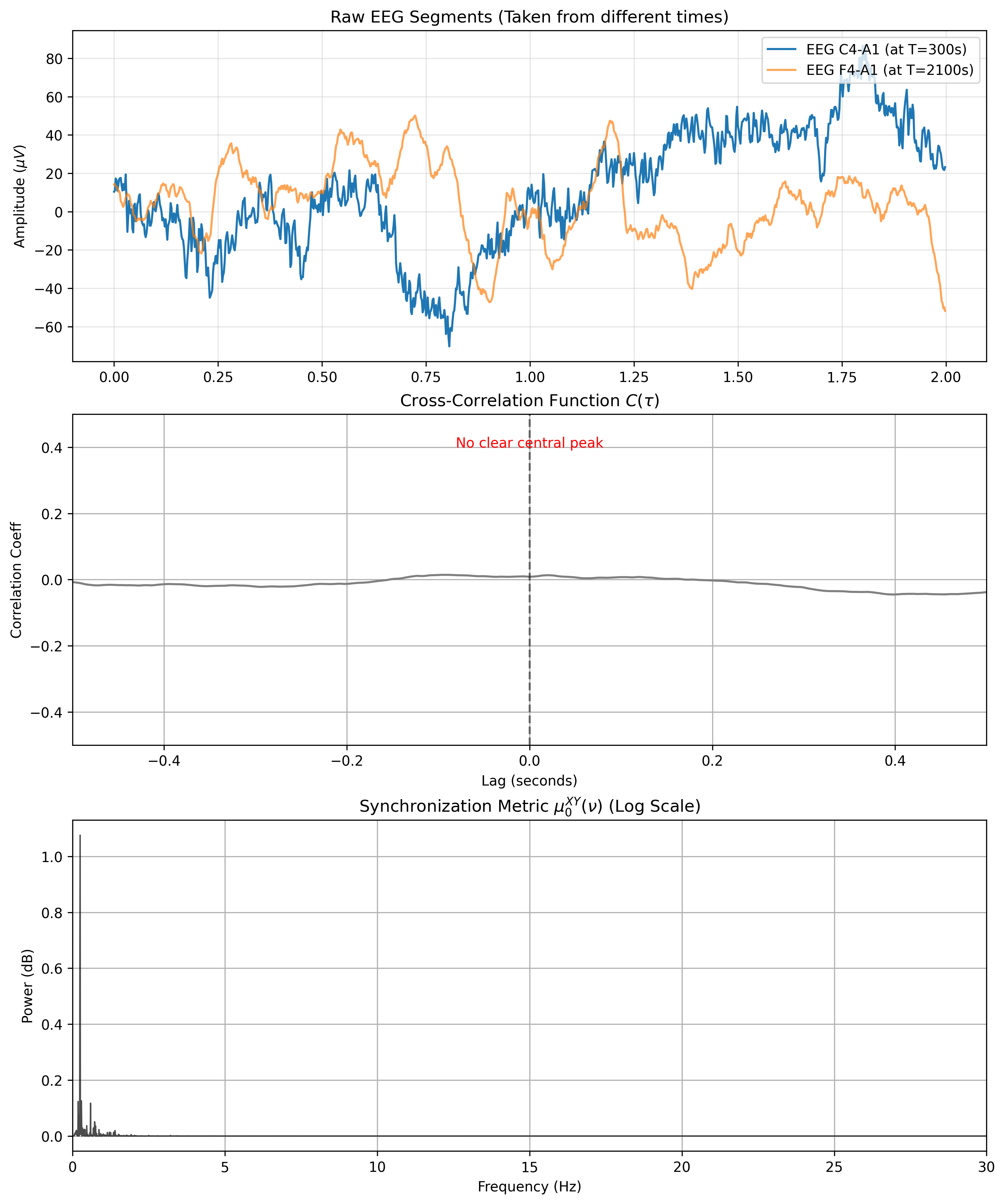
We see a close-to-flat cross-correlation, as expected, and very little power shared across frequencies.
Last note: frequencies below 0.3Hz are rather meaningless and typically removed. I also did not remove them for this example because (a) I am lazy and (b) the example still shows the point of the cross-spectrum neatly.
The matter does not end here and there is still some ground to cover. There is an argument to be made in favor of using not the co-spectrum but the quad-spectrum. In particular, perfect synchronicity between two brain regions might indicate not coordinated activity but rather the simultaneous reception of a signal from a third source. This is termed volume conduction and is considered an artifact, because it creates spurious correlation between two records.
For this reason, an alternative strategy is to ignore not the quad-spectrum but the co-spectrum all-together. For instance, this is the purpose of what is termed weighted Phase Lag Index (wPLI).
The wPLI ignores the magnitude of the delay and looks only at the asymmetry of the phase distribution across many observations. To compute it, we split our signals into $N$ smaller time segments (epochs). Let $k$ denote the $k$-th segment. The wPLI is defined is defined as
$$ \text{wPLI} = \frac{ | \sum_{k=1}^N \text{Quad-spectrum}_k | }{ \sum_{k=1}^N | \text{Quad-spectrum}_k | } $$
is more generally written as
$$ \text{wPLI} = \frac{ | \langle \Im(S_{XY}) \rangle | }{ \langle | \Im(S_{XY}) | \rangle } = \frac{ | \sum_{k=1}^N \Im(S_{XY})_k | }{ \sum_{k=1}^N | \Im(S_{XY})_k | } $$
The denominator ensures that $\text{wPLI} \in[0, 1]$ and is thus a normalization factor.
Using wPLI ensures that if quad-spectrum is very small (meaning the phase difference is very close to zero), we don't let it vote as strongly as a clear, large-magnitude phase lag. This effectively avoids the issue of volume conduction. Most serious papers use the wPLI and one could say that co-spectrum-based measures of connectivity are more or less deprecated.
To demonstrate the utility of the wPLI, I simulated two scenarios in Julia. I generated paired signals $X, Y$ representing 50 distinct epochs of 2 seconds each, sampled at 250 Hz. Both signals were constructed based on a shared 10 Hz oscillation modeled as:
$$X(t) = \sin(2\pi f t + \theta_{jitter}) + \mathcal{N}(0, 0.5)$$
$$Y(t) = \sin(2\pi f t + \theta_{jitter} + \phi_{lag}) + \mathcal{N}(0, 0.5)$$
where $f=10$Hz is the target frequency, $\theta_{jitter}$ is a random phase
offset applied to both signals equally in each epoch, $\mathcal{N}(0, 0.5)$ is
Gaussian white, and $\phi_{lag}$ is the critical variable manipulated between
scenarios. One scenario had «true synchrony», i.e. non-zero phase lag
synchronyzation with $\phi_{lag} = \pi / 2$ (90 degrees). The other scenario
had $\phi_{lag} = 0$, simulating a spurious synchronyzation caused by volume
conduction. For each scenario, I used the compute_wpli function from my
EEGToolkit scientific
packakge to estimate wPLI between the simulated signals. These were the results:
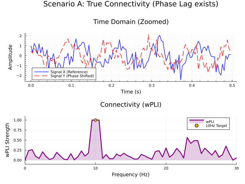
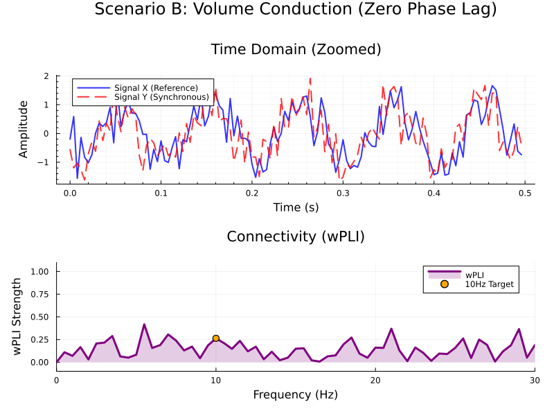
As we can see, in scenario $A$ (phase-lagged synchronyzation), the wPLI value is accurately capturing synchronyzation in the 10Hz rythm. In scenario $B$, though the signals are very similar, the fact that there is no phase lag makes the wPLI very low across all frequencies. Pretty interesting, huh?
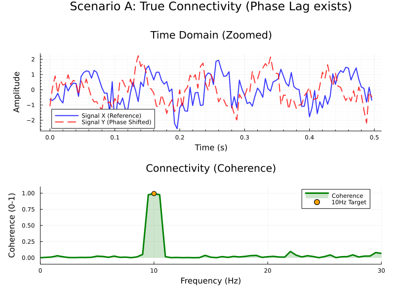
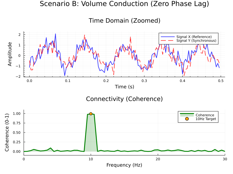
Just for fun, let us run the same simulations, but this time compute the magnitude-squared coherence (also implemented in my EEGToolkit package) instead of the wPLI.
$$C_{xy}(f) = \frac{|\langle S_{xy}(f) \rangle|^2}{\langle S_{xx}(f) \rangle \langle S_{yy}(f) \rangle}$$
This will serve us to illustrate the false positive problem which arises with volume conduction. The coherence will in fact detect the 10Hz synchronyzation in the phase-lagged scenario, which is correct. However, it will also detected for the zero-lag synchronyzation, which most likely is due to volume conduction. Importantly, there is no way to determine when coherence measures come from volume conduction as opposed to true synchronyzation.