Imagine you have a dataset that is high-dimensional and highly structured. A classic example is EEG data: you have $k = 64$ electrodes placed across the scalp, and perhaps you have used them to measure brain connectivity. You've done this for $g_1$ members of a certain group and $g_2$ members of another, so that you effectively have two $k \times g_1$ and $k \times g_2$ matrices with the resulting values. You ask the question: are the members of group 1 significantly different from the members of group 2?
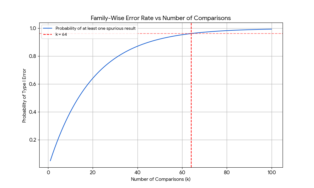
The naïve approach is to perform a $t$-test for every single electrode (i.e. every single row). But then the good old multiple comparisons problem creeps in, and you are either left exceedingly happy by the conclusivness of your findings, or doubting something fishy is going on. Indeed, if you run $k$ statistical tests with a standard significance level of $\alpha = 0.05$, and $k$ is sufficiently high, you are almost guaranteed to find spuriously significant results by chance. This is given by:
$$ P(\text{Number of Type I errors } \geq 1) = 1 - (1-\alpha)^k $$
which is plotted below as a function of $k$.
A point of confusion when first learning of the multiple comparisons problem, at least for me, was that intuitively one should think that more data should not lead to a greater chance of error. But data is typically two-dimensional: we have a number of features or variables, each with a sample size. Increasing the sample size is good. The multiple comparison problem arises when we increase the number of features. In our example, this would be the number of EEG electrodes.
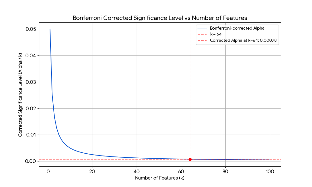
There are general forms of addressing this problem, where by general I mean that they do not leverage domain specific knowledge about the data and are thus agnostic about its properties. An example is Bonferroni correction, which simply divides the significant level $\alpha$ by the number of features $k$. However, these strategies are usually too harsh. The plot below shows how the Bonferroni-corrected significance level decays as $k$ increses, becoming $\alpha' = \alpha/64 = 0.00078$ for $k=64$. Thus, in addressing Type I errors (false positives), it increases the risk of Type II errors (false negatives) by making the significance threshold too strict.
Agnosticism is good, but the approach we hereby presents makes use of certain properties specific to the data—properties which are typical in biological studies. I am speaking of statistical dependence between spatially proximate features. Again, EEG is a good example: EEG electrodes are topologically related. If an electrode over the frontal lobe is highly active, a neighboring electrode will probably show similar activity.
Whenever some adequate sense of relatedeness or hubeness appears, it means our problem might be suited for a graph or network representation. Instead of asking «is this data point significantly different between groups», it might make more sense to ask: «is this region of points significantly different between groups», where this «regionness» is properly defined.
It should be clear that when shifting our view from points to regions or, as we will call them from now on, clusters, reduces the number of data points. We are in a sense lowering the data resolution, performing dimensionality reduction in view of real-world considerations. This not only controls the false alarm rate but improves sensitivity: if it is true that our data represents a topologically dependent system, where activity and inactivity are to be measured in terms of regions and not of points, then effects that are weaker at single points but strong in the region will be detected. Furthermore, and again assuming our topological considerations are true, single points showing exceedingly low or high activity relative to its surrounding are most likely spurious artifacts, and cluster based methods will effectively ignore them.
So far I have only provided an intuition, but we have to be more concrete. Once we see our data from a topological sense, as a graph or a network, how do we find clusters? What is a cluster and what isn't? How do we determine a node's belonging to a given cluster?
The statistical technique I will present is called cluster-based permutation testing. It models the $k$ features (e.g. the $k$ EEG electrodes) as real-valued nodes in a graph, where two nodes are connected if the features they represent are topologically related. Then it performs the following steps:
(1) For each feature, run a statistical test between the two groups. The choice of the test is a matter of debate, as seen in the paper above, but let us assume we have ran a $t$-test and thus, for each of the $k$ features, we have a $T$-statistic.
In our example, this would mean that, for each EEG electrode in the scalp, we would be able to say: according to a standard $t$-statistic, the activity of this electrode is/is not significantly different between the two groups.
(2) Mask the features (or nodes) whose statistic exceeded the threshold of statistical significance.
(3) From each masked node that is not yet in a cluster, form a cluster performing BFS and finding masked neighbours. If the initial masked node had no masked neighbours, then it will not form a cluster.

(4) For each cluster, compute some measure of the statistical strength in that cluster. Typically, the sum of the statistics of each node within it.
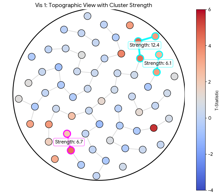
We now have clusters with an adequate notion of strength, but how do we produce a sound statistical analysis of them? If we have a cluster with a "mass" (sum of $t$-statistics) of, say, $T_{obs} = 50$, is that high or low? Is it rare or usual? Since the shape of our clusters is determined by the data itself, there is no standard distribution that can tell us the probability of observing a cluster mass of any given mass. We must construct the distribution ourselves using the null hypothesis.
The null hypothesis states that there is no difference between the groups. If this is true, the labels "Group 1" and "Group 2" are meaningless; we could shuffle the participants between the groups, and it shouldn't change the result.
To test this, we perform the following Monte Carlo permutation, which is step (5).
-
Shuffling: Take all $g_1 + g_2$ participants, pool them together, and randomly assign them to two new groups of size $g_1$ and $g_2$.
-
Recalculate: Run the exact same steps as before (Steps 1 through 4). Perform the $t$-tests for every electrode, threshold them, find clusters, and sum their $t$-statistics.
-
Find the Maximum: Record only the maximum cluster statistic found in the iteration. By tracking the single largest cluster that arises purely by chance in each iteration, we control the Family-Wise Error Rate (FWER). We are effectively building a distribution of "the worst false positives that could happen by chance.
-
Repeat: Repeat this shuffling process $N$ with $N$ sufficiently large.
This produces a distribution of maximum cluster masses under the null hypothesis. All that is left is to compute the $p$-value.
The simulated $p$-value is simply the proportion of random permutations that produced a cluster mass greater than or equal to the empirical mass in our data:
$$ p =\frac{\text{count}(T_{perm} \geq T_{obs})}{N} $$
If our empirical cluster is larger than 95% of the maximum clusters found by chance ($p < 0.05$), the null hypothesis is rejected and we can conclude that there is a significant difference between the groups.